Divisibility of Separated Polynomials

The mechanism

Choose a module basis that exposes composition

A divisibility condition in two variables can conceal a one-variable composition. The proof expands in a suitable free-module basis and compares the surviving coefficients along the diagonal. The new working coordinates isolate the restriction imposed by divisibility.

What becomes elementary: A polynomial divisibility question becomes a controlled remainder and coefficient calculation.

Read the free-module proof and work through the extraction example. The Galois and Frobenius companion in the Tensorgami archive supplies a second route with its own hypotheses; compare which work each representation makes immediate.

Explore further constructions. Edition dates, sources and reference chapters identify the scope of each study.

Overview

Let $k$ be a field and let $f,g,p,q\in k[t]$ , with $f$ and $g$ nonconstant. We prove that

f(x)-g(y)\mid p(x)-q(y) \quad \text{in } k[x,y]

if and only if there is a single polynomial

s\in k[t]

such that

p=s\circ f, \qquad q=s\circ g.

The proof uses the fact that

k[x]

is a free

k[f]

-module with basis

1,x,\dots,x^{\deg f-1}

, and then applies this independently in the two variables. The resulting residue rectangle in

k[x,y]

turns the divisibility hypothesis into coefficient identities in

k[U,V]

. The final step is the diagonal specialization

U=V

, equivalently reduction modulo

U-V

. We also include an explicit algorithm for extracting the common outer polynomial and an application to a symmetric functional equation whose branches come from the fibers of

t^3+t

1 · Statement and first comments

Separated polynomials, namely polynomials of the form $p(x)-q(y)$ , occur naturally in factorization problems, fiber products of polynomial maps, and functional equations with conjugate branches. The following theorem says that divisibility by another separated polynomial $f(x)-g(y)$ is rigid: it occurs exactly when $p$ and $q$ both descend from the same one-variable polynomial on the common value of $f$ and $g$ .

Theorem 1.1 (Separated divisibility criterion). Let $k$ be a field, and let
$f,g,p,q\in k[t], \qquad \deg f>0, \qquad \deg g>0.$ Then $f(x)-g(y)\mid p(x)-q(y) \qquad \text{in } k[x,y]$ if and only if there exists $s\in k[t]$ such that $p(t)=s(f(t)), \qquad q(t)=s(g(t)).$

The reverse implication is immediate. If $p=s\circ f$ and $q=s\circ g$ , then

p(x)-q(y)=s(f(x))-s(g(y)).

For every polynomial

s

, the difference

s(U)-s(V)

is divisible by

U-V

k[U,V]

, so after substituting

U=f(x), \qquad V=g(y),

we get

f(x)-g(y) \mid s(f(x))-s(g(y)) =p(x)-q(y).

The forward implication is the substantial part.

2 · The one-variable free-module expansion

We first isolate the basic one-variable fact. It is useful to state it over a general integral domain, because in the two-variable proof the coefficient ring will temporarily be $k[y]$ or $k[U]$ .

Lemma 2.1 (One-variable residue expansion). Let $R$ be an integral domain, and let
$F(t)=\lambda t^d+\alpha_{d-1}t^{d-1}+\cdots+\alpha_0\in R[t],$ where $d>0$ and $\lambda\in R^\times$ . Then $R[t] = \bigoplus_{i=0}^{d-1} R[F]t^i.$ Equivalently, every $H(t)\in R[t]$ has a unique expression $H(t)=\sum_{i=0}^{d-1} A_i(F(t))t^i, \qquad A_i\in R[T].$

Proof. Since $\lambda$ is a unit in $R$ , we may solve for $t^d$ :

t^d = \lambda^{-1}F(t) - \lambda^{-1}\sum_{r=0}^{d-1}\alpha_r t^r.

This identity reduces the power

t^d

to an

R[F]

-linear combination of

1,t,\dots,t^{d-1}.

Multiplying by powers of

t

and arguing by induction, every monomial

t^N

belongs to

\sum_{i=0}^{d-1} R[F]t^i.

Therefore the displayed sum spans

R[t]

For uniqueness, suppose

\sum_{i=0}^{d-1} A_i(F(t))t^i=0, \qquad A_i\in R[T].

Assume some

A_i

is nonzero. For each nonzero

A_i

, write

A_i(T)=a_i T^{e_i}+\text{lower powers of }T, \qquad a_i\neq 0.

Since

R

is an integral domain and

\lambda

is a unit, the leading term of

A_i(F(t))t^i

has degree

d e_i+i.

For distinct

i\in\{0,\dots,d-1\}

, the integers

d e_i+i

lie in distinct congruence classes modulo

d

. Hence among the nonzero summands there is a unique summand of largest

t

-degree. Its leading term cannot cancel with anything else. This contradicts the equality to zero.

Thus all $A_i$ vanish, and the expansion is unique. ◻

Remark 2.2 (No monicity needed). The polynomial $F$ need not be monic. We only need its leading coefficient to be a unit. In the main theorem the coefficient ring is a field, so every nonzero leading coefficient is automatically a unit.

Corollary 2.3. Let $k$ be a field and let $f\in k[t]$ have degree $n>0$ . Then
$k[x] = \bigoplus_{i=0}^{n-1} k[f(x)]x^i.$ In particular, every $p(x)\in k[x]$ has a unique expression $p(x)=\sum_{i=0}^{n-1} a_i(f(x))x^i, \qquad a_i\in k[T].$

3 · The two-variable residue rectangle

Set

n=\deg f, \qquad m=\deg g.

The next proposition is the structural heart of the proof.

Proposition 3.1 (Two-variable residue expansion). Let $f,g\in k[t]$ have degrees $n>0$ and $m>0$ , respectively. Then every polynomial $H(x,y)\in k[x,y]$ admits a unique expression
$H(x,y) = \sum_{0\leq i<n,\;0\leq j<m} C_{ij}(f(x),g(y))x^i y^j,$ where $C_{ij}(U,V)\in k[U,V].$ Equivalently, $k[x,y] = \bigoplus_{0\leq i<n,\;0\leq j<m} k[f(x),g(y)]x^i y^j.$ Thus $k[x,y]$ is a free $k[f(x),g(y)]$ -module of rank $nm$ , with basis $\mathcal B= \{x^i y^j:0\leq i<n, \;0\leq j<m\}.$

Proof. We first prove existence. Regard $k[x,y]$ as $k[y][x]$ . Applying Lemma 2.1 with coefficient ring $R=k[y]$ and polynomial $f(x)$ , we can write

H(x,y) = \sum_{i=0}^{n-1} A_i(f(x),y)x^i,

where

A_i(U,y)\in k[U,y].

Now fix

i

. Regard

A_i(U,y)

as a polynomial in

y

with coefficients in the integral domain

k[U]

. Applying Lemma 2.1 again, now with polynomial

g(y)

, gives

A_i(U,y) = \sum_{j=0}^{m-1} C_{ij}(U,g(y))y^j,

for some

C_{ij}(U,V) \in k[U,V].

Substituting

U=f(x)

yields the desired expression.

For uniqueness, suppose

\sum_{0\leq i<n,\;0\leq j<m} C_{ij}(f(x),g(y))x^i y^j=0.

For each

i

, put

B_i(U,y) = \sum_{j=0}^{m-1} C_{ij}(U,g(y))y^j \in k[U,y].

Then

\sum_{i=0}^{n-1} B_i(f(x),y)x^i=0.

By Lemma 2.1, applied over the coefficient ring

k[y]

, each polynomial

B_i(U,y)

is zero. Hence, for each

i

\sum_{j=0}^{m-1} C_{ij}(U,g(y))y^j=0 \qquad \text{in } k[U,y].

Applying Lemma 2.1 again over the coefficient ring

k[U]

, we obtain

C_{ij}(U,V)=0

for every pair

(i,j)

. This proves uniqueness. ◻

Remark 3.2 (Lattice intuition). The uniqueness says that the monomials $x^i y^j$ with
$0\leq i<n, \qquad 0\leq j<m$ form a fundamental residue rectangle. Multiplication by powers of $f(x)$ and $g(y)$ moves this rectangle by degree increments of size $n$ in the $x$ -direction and size $m$ in the $y$ -direction. The formal proof above avoids choosing a monomial order, but the following picture captures the degree geometry.

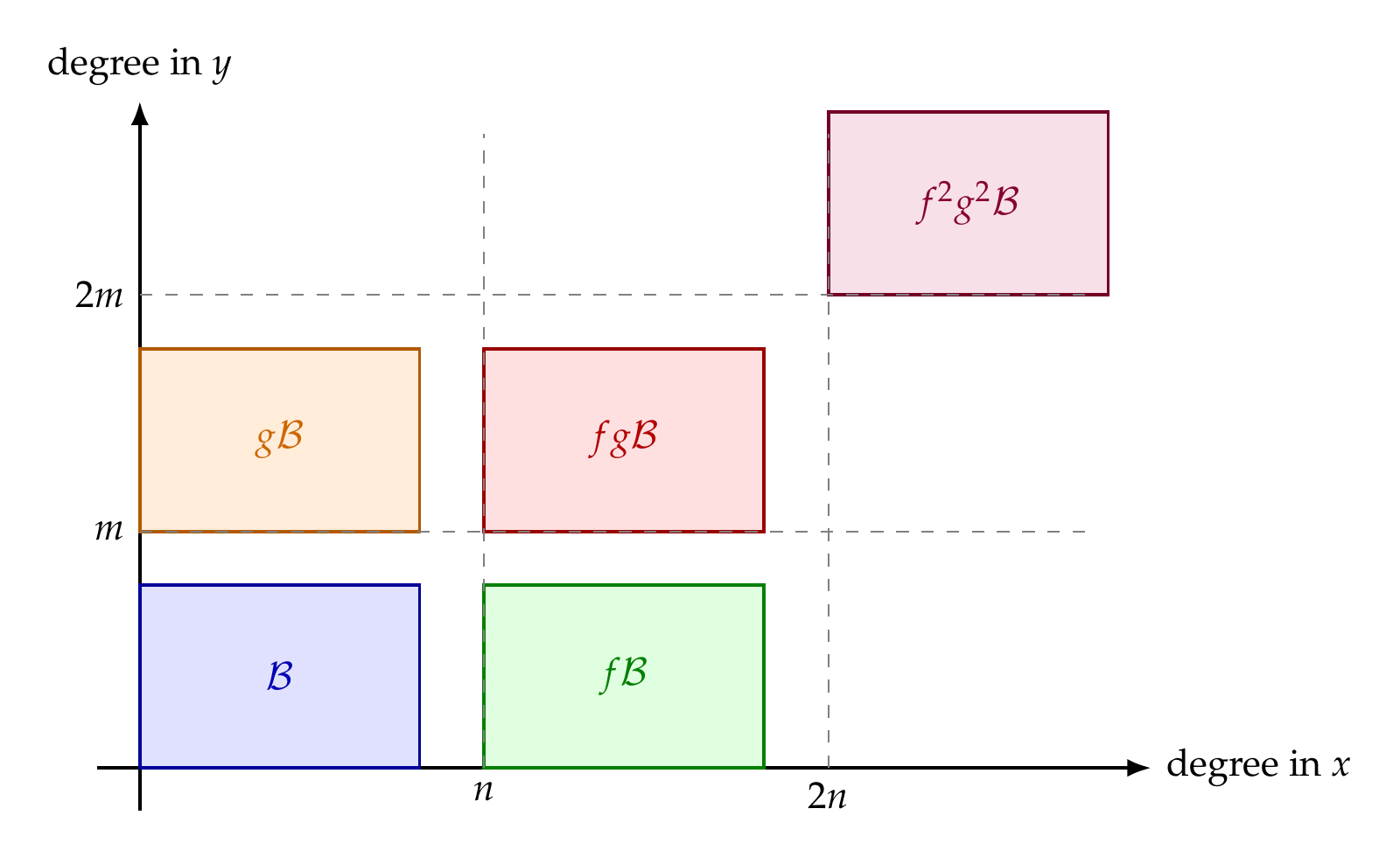
A degree lattice with the residue rectangle B and its translated rectangles f B, g B, f g B, and f squared g squared B. — The residue rectangle $\mathcal B$ and some of its degree shifts under multiplication by $f(x)$ and $g(y)$ .

Corollary 3.3 (Algebraic independence). The natural homomorphism
$k[U,V] \longrightarrow k[x,y], \qquad U\longmapsto f(x), \qquad V\longmapsto g(y),$ is injective. Equivalently, $f(x)$ and $g(y)$ are algebraically independent over $k$ .

Proof. If $C(f(x),g(y))=0$ , then this is a residue expansion supported only in the $(i,j)=(0,0)$ slot. By uniqueness in Proposition 3.1, $C=0$ . ◻

4 · Proof of the divisibility criterion

We now prove Theorem 1.1.

Assume

f(x)-g(y) \mid p(x)-q(y) \qquad \text{in } k[x,y].

Then there exists

H(x,y)\in k[x,y]

such that

p(x)-q(y)=(f(x)-g(y))H(x,y).

By Proposition 3.1, write

H(x,y) = \sum_{0\leq i<n,\;0\leq j<m} C_{ij}(f(x),g(y))x^i y^j,

where

C_{ij}\in k[U,V]

. Then

(f(x)-g(y))H(x,y) = \sum_{0\leq i<n,\;0\leq j<m} (U-V)C_{ij}(U,V)\big|_{U=f(x),\,V=g(y)}x^i y^j.

On the other hand, by Corollary 2.3, the polynomials $p$ and $q$ have unique expansions

p(x)=\sum_{i=0}^{n-1} a_i(f(x))x^i, \qquad a_i\in k[U],

and

q(y)=\sum_{j=0}^{m-1} b_j(g(y))y^j, \qquad b_j\in k[V].

Therefore the two-variable residue expansion of

p(x)-q(y)

p(x)-q(y) = a_0(f(x))-b_0(g(y)) + \sum_{i=1}^{n-1}a_i(f(x))x^i - \sum_{j=1}^{m-1}b_j(g(y))y^j.

Comparing the unique coefficients in the residue rectangle gives identities in $k[U,V]$ :

\begin{align} (U-V)C_{ij}(U,V)&=0 &&\text{for } i>0, \;j>0, \tag{1}\\ (U-V)C_{i0}(U,V)&=a_i(U) &&\text{for } i>0, \tag{2}\\ (U-V)C_{0j}(U,V)&=-b_j(V) &&\text{for } j>0, \tag{3}\\ (U-V)C_{00}(U,V)&=a_0(U)-b_0(V). \tag{4} \end{align}

The comparison can be visualized as follows: the right-hand side $p(x)-q(y)$ occupies only the bottom row and the left column of the residue rectangle, while the product $(f(x)-g(y))H(x,y)$ has coefficient $(U-V)C_{ij}$ in every slot.

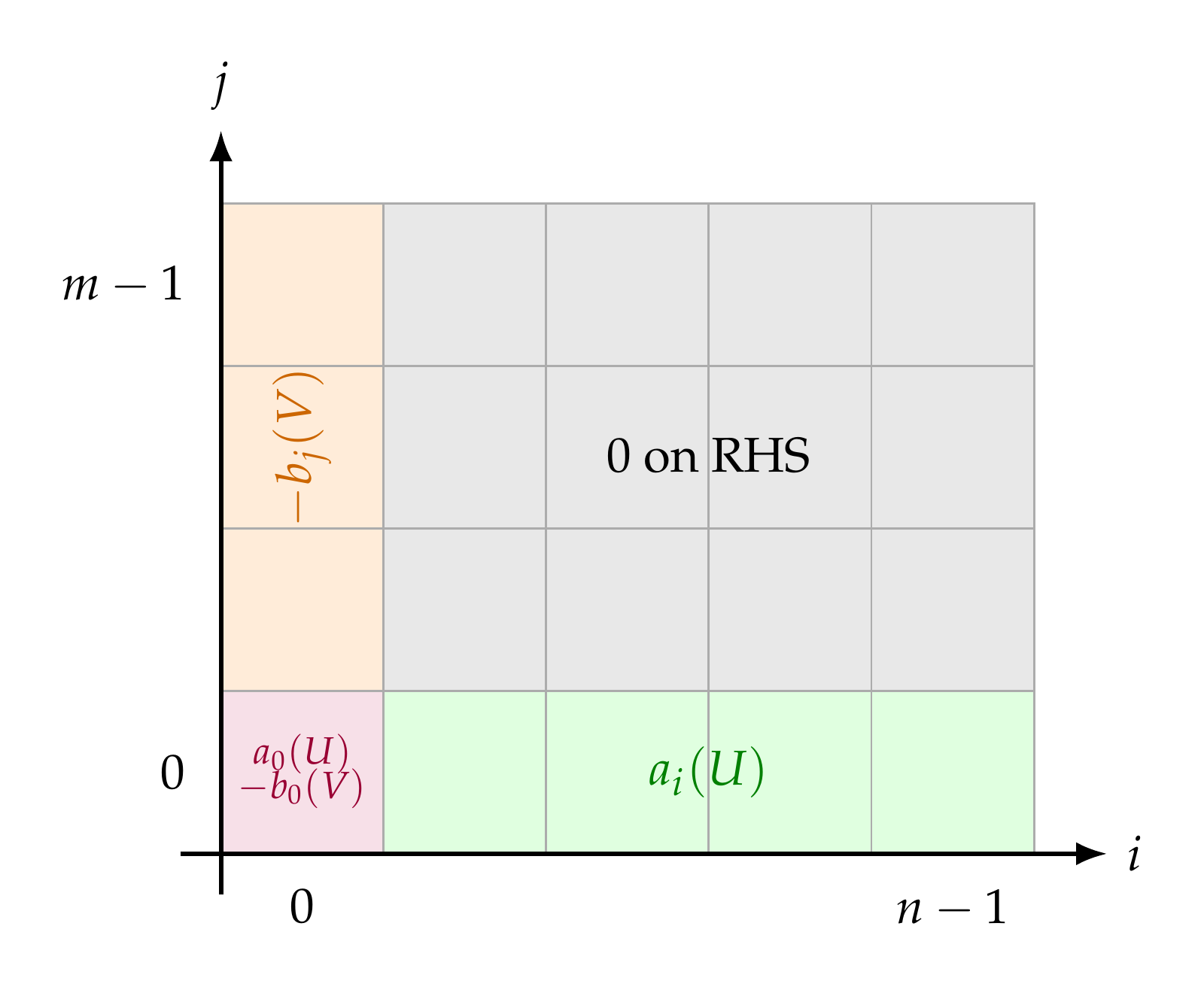
The coefficient rectangle: the bottom row contains a i of U, the left column contains minus b j of V, the origin contains a zero of U minus b zero of V, and the remaining entries are zero. — The coefficient comparison in the residue rectangle.

Since $k[U,V]$ is an integral domain and $U-V\neq 0$ , equation (1) gives

C_{ij}=0 \qquad \text{for } i>0, \;j>0.

Now consider the diagonal specialization map

\Delta:k[U,V]\longrightarrow k[T], \qquad \Delta(U)=T, \qquad \Delta(V)=T.

This is the same as reducing modulo the ideal

(U-V)

Applying $\Delta$ to equation (2) gives

0=a_i(T) \qquad \text{for } i>0.

Thus

a_i=0 \qquad \text{for } i>0.

Then equation (2) also gives

C_{i0}=0

for

i>0

Similarly, applying $\Delta$ to equation (3) gives

0=-b_j(T) \qquad \text{for } j>0,

b_j=0 \qquad \text{for } j>0.

Then equation (3) also gives

C_{0j}=0

for

j>0

Finally, applying $\Delta$ to equation (4) gives

0=a_0(T)-b_0(T).

Hence

a_0=b_0 \qquad \text{in } k[T].

Define

s(T)=a_0(T)=b_0(T).

Since all

a_i

for

i>0

vanish, the expansion of

p

reduces to

p(x)=a_0(f(x))=s(f(x)).

Since all

b_j

for

j>0

vanish, the expansion of

q

reduces to

q(y)=b_0(g(y))=s(g(y)).

Replacing

x

and

y

by a single indeterminate

t

, we get

p(t)=s(f(t)), \qquad q(t)=s(g(t)).

This proves the forward implication.

For the converse, suppose $p=s\circ f$ and $q=s\circ g$ . Write

s(T)=\sum_{\ell=0}^N c_\ell T^\ell.

Then

s(U)-s(V) = \sum_{\ell=1}^N c_\ell(U^\ell-V^\ell) = (U-V) \sum_{\ell=1}^N c_\ell\sum_{r=0}^{\ell-1}U^{\ell-1-r}V^r.

Thus

U-V\mid s(U)-s(V)

. Substituting

U=f(x)

and

V=g(y)

gives

f(x)-g(y) \mid s(f(x))-s(g(y)) = p(x)-q(y).

The theorem follows. ◻

5 · The binomial-shift version of the diagonal step

The diagonal map $\Delta$ is the shortest way to express the last step of the proof. It is also useful to spell out the equivalent constructive version, because it explains exactly how terms are moved into a multiple of $U-V$ .

Lemma 5.1 (Binomial shift). For every $B(T)\in k[T]$ , there is a polynomial $Q_B(U,V)\in k[U,V]$ such that
$B(V)=B(U)+(V-U)Q_B(U,V).$ More explicitly, if $B(T)=\sum_{\ell=0}^N c_\ell T^\ell,$ then one may take $Q_B(U,V) = \sum_{\ell=1}^N c_\ell \sum_{r=0}^{\ell-1} V^{\ell-1-r}U^r.$

Proof. Use

V^\ell-U^\ell = (V-U)\sum_{r=0}^{\ell-1}V^{\ell-1-r}U^r

for every

\ell\geq 1

, and sum over the terms of

B

. ◻

Applying this lemma to $B=b_0$ , equation (4) becomes

(U-V)C_{00}(U,V) = a_0(U)-b_0(U)+(U-V)Q_{b_0}(U,V).

Equivalently,

(U-V)\bigl(C_{00}(U,V)-Q_{b_0}(U,V)\bigr) = a_0(U)-b_0(U).

Reducing modulo

U-V

, or equivalently setting

V=U

, forces

a_0(U)-b_0(U)=0.

This is precisely the same argument as the diagonal specialization, written in expanded binomial form.

6 · Algorithmic extraction of the outer polynomial

Once $P=S\circ G$ is known, division by $G(t)-Z$ recovers $S$ as a remainder. The same division also tests whether such an $S$ exists.

Proposition 6.1 (Remainder extraction). Let $G(t),P(t)\in k[t]$ , with $d=\deg G>0$ , and let $Z$ be a new indeterminate. Divide $P(t)$ , as a polynomial in $t$ , by $G(t)-Z$ over the coefficient ring $k[Z]$ :
$P(t)=A(t,Z)(G(t)-Z)+R(t,Z), \qquad \deg_t R<d.$ Then $P\in k[G]$ if and only if the remainder $R(t,Z)$ is independent of $t$ , i.e. $R(t,Z)\in k[Z]$ . In that case $P(t)=R(G(t))$ and $R(Z)$ is the unique outer polynomial.

In particular, if it is already known that $P(t)=S(G(t))$ , then the remainder is exactly
$R(t,Z)=S(Z).$

Proof. The division is valid in $k[Z][t]$ because the leading coefficient of $G(t)-Z$ , viewed as a polynomial in $t$ , is the nonzero leading coefficient of $G$ , hence a unit of $k[Z]$ .

Suppose first that $P(t)=S(G(t))$ . In $k[X,Z]$ , the difference $S(X)-S(Z)$ is divisible by $X-Z$ , so there exists $B(X,Z)\in k[X,Z]$ such that

S(X)-S(Z)=(X-Z)B(X,Z).

Substituting

X=G(t)

gives

P(t)=S(G(t))=(G(t)-Z)B(G(t),Z)+S(Z).

Since

S(Z)

is independent of

t

and

d>0

, uniqueness of division by

G(t)-Z

gives

R(t,Z)=S(Z).

Conversely, suppose the remainder is independent of $t$ , say $R(t,Z)=S(Z)$ . Apply the homomorphism

k[Z,t]\longrightarrow k[t], \qquad Z\longmapsto G(t), \qquad t\longmapsto t.

The division identity becomes

P(t)=A(t,G(t))(G(t)-G(t))+S(G(t))=S(G(t)).

Thus

P\in k[G]

Finally, uniqueness of $S$ follows from injectivity of

k[Z]\longrightarrow k[t], \qquad Z\longmapsto G(t),

which is immediate from

\deg G>0

: if

S\neq 0

, then

S(G(t))\neq 0

and has degree

(\deg S)(\deg G)

. ◻

Remark 6.2 (Using the extraction after Theorem 1.1). If
$f(x)-g(y) \mid p(x)-q(y),$ then Theorem 1.1 guarantees $p=s\circ f$ and $q=s\circ g$ . Proposition 6.1 recovers $s$ by dividing $p(t)$ by $f(t)-Z$ , or equivalently by dividing $q(t)$ by $g(t)-Z$ . The two remainders must agree, and their common value is $s(Z)$ .

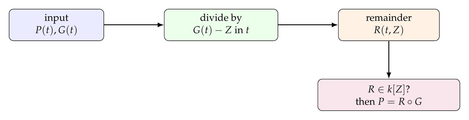
Remainder extraction: divide P of t by G of t minus Z in t, obtain R of t and Z, and test whether the remainder is independent of t. — Remainder extraction: the outer polynomial is the $t$ -constant remainder after division by $G(t)-Z$ .

A worked extraction and a failed test

Over $\mathbb Q$ , take

f(t)=t^2,\qquad g(t)=t^3,\qquad p(t)=t^4+2t^2,\qquad q(t)=t^6+2t^3.

To test

p

against

f

, divide by

t^2-Z

t^4+2t^2=(t^2+Z+2)(t^2-Z)+(Z^2+2Z).

The remainder is independent of

t

, so the recovered outer polynomial is

s(Z)=Z^2+2Z

. The same calculation with

q

gives

t^6+2t^3=(t^3+Z+2)(t^3-Z)+(Z^2+2Z).

Both remainders agree. In the original two variables the certificate is

p(x)-q(y)=(x^2-y^3)(x^2+y^3+2).

For a failed test, keep

f(t)=t^2

but replace

p(t)

t^3

. Now

t^3=t(t^2-Z)+Zt.

The remainder

Zt

still depends on

t

, so

t^3\notin\mathbb Q[t^2]

. The algorithm thus supplies either the common outer polynomial or a concrete remainder showing why descent fails.

7 · Quotient-ring interpretation

Let

A=k[x,y]/(f(x)-g(y)),

and write bars for images in

A

. In

A

, the defining relation is

\overline{f(x)}=\overline{g(y)}.

The theorem can be rephrased as the intersection identity

\overline{k[x]}\cap \overline{k[y]} = k[\overline{f(x)}] = k[\overline{g(y)}] \subseteq A.

Indeed, if an element of

\overline{k[x]}\cap \overline{k[y]}

is represented both by

p(x)

and by

q(y)

, then

p(x)-q(y)\in (f(x)-g(y)).

By Theorem 1.1, there is

s\in k[t]

such that

p=s\circ f, \qquad q=s\circ g.

Thus the common element is

s(\overline{f(x)})=s(\overline{g(y)})

On the fiber product defined by

f(x)=g(y),

any function depending only on

x

and also only on

y

must come from the shared base coordinate.

8 · Geometric reading

Suppose, for intuition, that $k$ is algebraically closed. The equation

f(x)=g(y)

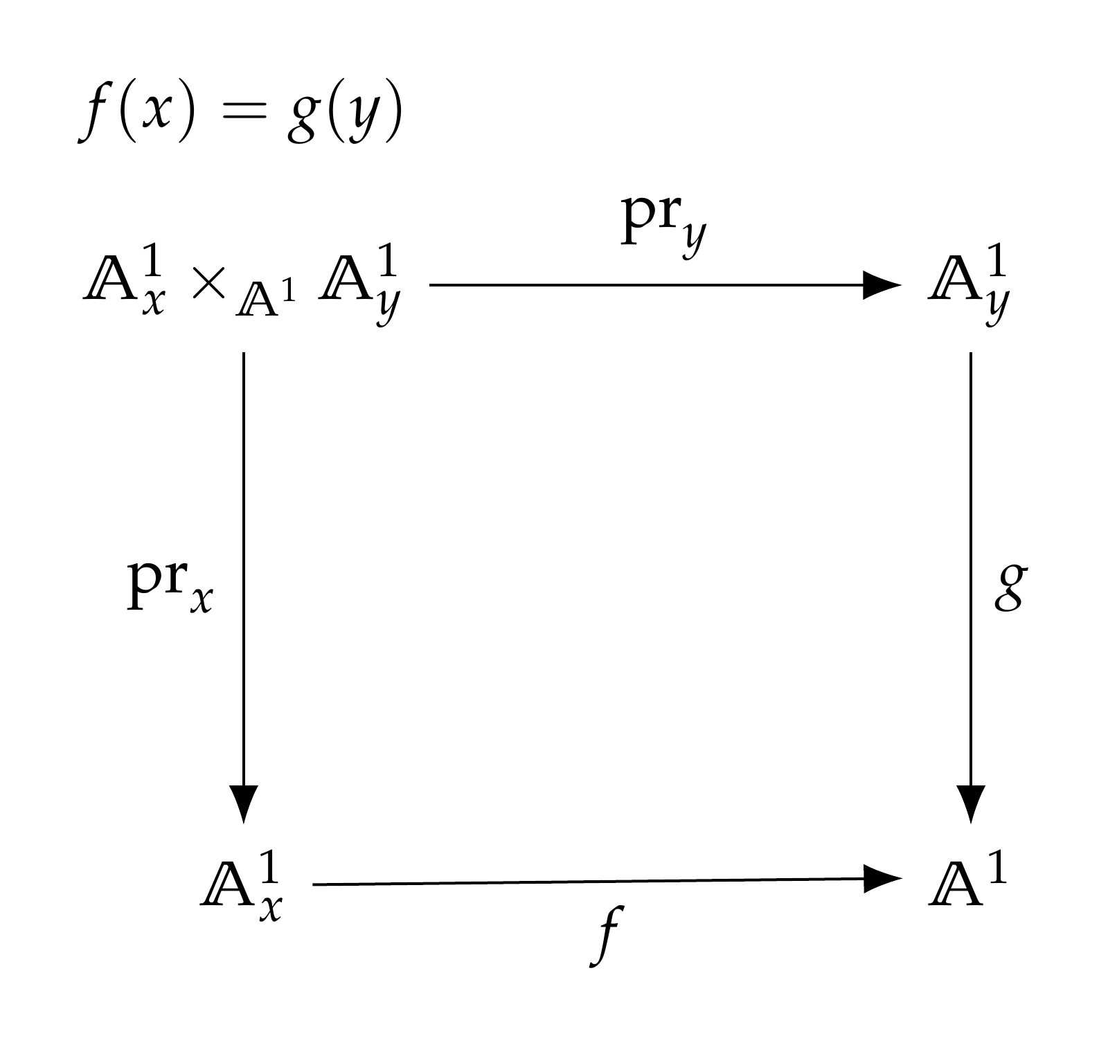
defines the fiber product of the maps

\mathbb A^1_x\longrightarrow \mathbb A^1, \qquad x\longmapsto f(x),

and

\mathbb A^1_y\longrightarrow \mathbb A^1, \qquad y\longmapsto g(y).

The divisibility condition

f(x)-g(y)\mid p(x)-q(y)

means that the separated equation

p(x)=q(y)

holds scheme-theoretically on this fiber product. The theorem then says that

p

and

q

are obtained by applying the same polynomial

s

to the common base value.

The fiber-product square: the projections from the fiber product of the two affine lines commute with f and g to their shared base affine line.

The diagram is only schematic: the algebraic proof does not require irreducibility of $f(x)-g(y)$ , separability of $f$ or $g$ , or any assumption on the characteristic of $k$ .

9 · Application: a symmetric functional equation

The criterion is particularly efficient when a functional equation says that a polynomial is constant on several algebraic branches lying above the same value of another polynomial. The following example is a model case.

Proposition 9.1 (A three-branch symmetry). Assume $\operatorname{char} k\neq 2$ . Let $\Phi(T)\in k[T]$ . Let $X$ be an indeterminate, and let $\alpha,\beta$ be the two roots, in an algebraic closure of $k(X)$ , of
$Y^2+XY+X^2+1=0.$ Equivalently, in square-root notation, $\alpha=\frac{-X+\sqrt{-3X^2-4}}{2}, \qquad \beta=\frac{-X-\sqrt{-3X^2-4}}{2}.$ If $\Phi(\alpha)=\Phi(X) \qquad\text{and}\qquad \Phi(\beta)=\Phi(X)$ in the corresponding algebraic extension of $k(X)$ , then there exists $h(T)\in k[T]$ such that $\Phi(T)=h(T^3+T).$ Conversely, every polynomial of the form $h(T^3+T)$ satisfies these two branch identities.

Proof. Put

G(T)=T^3+T.

A direct factorization gives

G(Y)-G(X) = (Y^3+Y)-(X^3+X) = (Y-X)(Y^2+XY+X^2+1).

Thus

Y=X

Y=\alpha

, and

Y=\beta

are the three roots of

G(Y)-G(X)=0

over an algebraic closure of

k(X)

These three roots are distinct. The quadratic factor is separable because its discriminant is

X^2-4(X^2+1)=-3X^2-4,

which is a nonzero element of

k(X)

when

\operatorname{char} k\neq 2

. Also,

Y-X

and

Y^2+XY+X^2+1

are coprime in

k(X)[Y]

, since substituting

Y=X

into the quadratic gives

3X^2+1,

which is nonzero in

k(X)

in all characteristics, including characteristic

3

, where it equals

1

By hypothesis,

\Phi(\alpha)-\Phi(X)=0, \qquad \Phi(\beta)-\Phi(X)=0,

and trivially

\Phi(X)-\Phi(X)=0.

Therefore the polynomial

\Phi(Y)-\Phi(X)\in k[X,Y]

vanishes at all three distinct roots of

G(Y)-G(X)

, viewed as a polynomial in

Y

over

k(X)

Since $G(Y)-G(X)$ is monic of degree $3$ in $Y$ , divide $\Phi(Y)-\Phi(X)$ by $G(Y)-G(X)$ in $k[X][Y]$ :

\Phi(Y)-\Phi(X) = Q(X,Y)(G(Y)-G(X))+R(X,Y), \qquad \deg_Y R<3.

The remainder

R

, considered in

k(X)[Y]

, also vanishes at the three distinct roots of

G(Y)-G(X)

. Since

\deg_Y R<3

, it must be zero. Hence

G(Y)-G(X) \mid \Phi(Y)-\Phi(X) \qquad \text{in } k[X,Y].

Equivalently,

G(X)-G(Y) \mid \Phi(X)-\Phi(Y).

Applying Theorem 1.1 with

f=g=G, \qquad p=q=\Phi,

we obtain a polynomial

h\in k[T]

such that

\Phi(T)=h(G(T))=h(T^3+T).

Conversely, if $\Phi(T)=h(G(T))$ , then whenever $G(Y)=G(X)$ , one has

\Phi(Y)=h(G(Y))=h(G(X))=\Phi(X).

In particular, the identities hold for the two branches

Y=\alpha

and

Y=\beta

. ◻

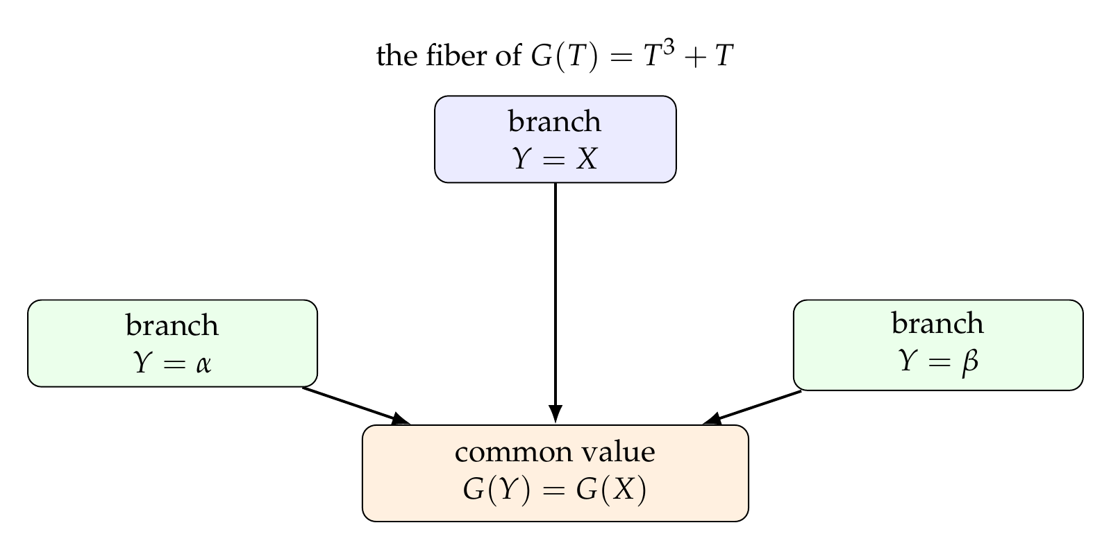
The three branches Y equals X, Y equals alpha, and Y equals beta map to the shared value G of Y equals G of X for G of T equals T cubed plus T. — The two conjugate branches and the trivial branch lie in the same fiber of $T^3+T$ .

Remark 9.2. The word “irreducible” is not needed in the argument. The quadratic branch polynomial may or may not be irreducible over $k(X)$ , depending on the field. What matters is that the three branches are distinct over an algebraic closure of $k(X)$ . The main divisibility criterion itself does not require any separability hypothesis; separability only enters here because we infer divisibility from vanishing at distinct branches.

10 · Fiber constancy in arbitrary characteristic

The preceding example uses distinct branches. For an arbitrary polynomial, the generic fiber can have multiplicities, and these must also be retained. The main theorem already handles them. The following consequence makes their role explicit without restricting the characteristic or assuming separability.

Let $G\in k[T]$ be nonconstant. In characteristic zero put $q=1$ and $H=G$ . In characteristic $p>0$ , let $q=p^e$ be the largest power of $p$ for which

G(T)=H(T^q),\qquad H\in k[T].

Thus

H'\ne0

. This decomposition simply groups the exponents of

G

; it does not require taking roots of its coefficients. Let

X

be indeterminate and let

\Omega

be an algebraic closure of

k(X)

For $\Phi\in k[T]$ , define its Hasse derivatives by the polynomial identity

\Phi(T+U)=\sum_{j\ge0}\partial^{[j]}\Phi(T)\,U^j.

In particular,

\partial^{[0]}\Phi=\Phi

. These coefficients record vanishing to a prescribed order in every characteristic.

Proposition 10.1 (Constancy with multiplicities). With the notation above, the following are equivalent:

$\Phi\in k[G]$ .

The classes of $\Phi(Y)$ and $\Phi(X)$ are equal in
$k[X,Y]/(G(Y)-G(X)).$

For every distinct root $\alpha\in\Omega$ of $G(Y)-G(X)$ ,
$\Phi(\alpha)=\Phi(X),\qquad \partial^{[j]}\Phi(\alpha)=0\quad(1\le j<q).$

Moreover, constancy on the geometric points alone has the exact characterization
$\Phi(\alpha)=\Phi(X)\ \text{for every such }\alpha \quad\Longleftrightarrow\quad \Phi(T)^q\in k[G].$

Proof. First, $H(Z)-G(X)$ has distinct roots over $\Omega$ . Indeed, a repeated root $\beta$ would satisfy $H'(\beta)=0$ , making $\beta$ , and hence $H(\beta)$ , algebraic over $k$ . This contradicts $H(\beta)=G(X)$ , since $G(X)$ is transcendental over $k$ .

For each root $\beta$ , the polynomial $Y^q-\beta$ has a unique root $\alpha$ in $\Omega$ and equals $(Y-\alpha)^q$ ; this includes the case $q=1$ . Consequently, for some $c\in k^\times$ ,

D(Y):=G(Y)-G(X)=c\prod_{\alpha}(Y-\alpha)^q,

where the roots in the product are distinct. Thus every point of the generic fiber has exactly the same multiplicity

q

Put $E(Y)=\Phi(Y)-\Phi(X)$ . Expanding $E(\alpha+U)$ , the Hasse derivative conditions in (3) say precisely that $(Y-\alpha)^q\mid E(Y)$ . The factors for distinct $\alpha$ are coprime, so (3) is equivalent to $D\mid E$ in $\Omega[Y]$ .

This divisibility descends to $k[X,Y]$ directly by polynomial division. The leading coefficient $c$ of $D$ lies in $k^\times$ , so division by $D$ in $k[X][Y]$ gives a remainder of $Y$ -degree less than $\deg G$ . Divisibility over $\Omega$ forces that same remainder to be zero. Hence (3) is equivalent to (2). Finally, the already proved Theorem 1.1, applied with $f=g=G$ and $p=q=\Phi$ in that theorem’s notation, gives (2) if and only if (1). No assertion about branches was used in its free-module proof.

For the last assertion, pointwise constancy makes each $(Y-\alpha)$ divide $E$ , hence makes $D$ divide $E^q$ . Since $q$ is a power of the characteristic, or $q=1$ ,

E(Y)^q=\Phi(Y)^q-\Phi(X)^q.

The same division argument and Theorem 1.1 give

\Phi(T)^q\in k[G]

. Conversely, if

\Phi(T)^q=S(G(T))

, then

G(\alpha)=G(X)

implies

\Phi(\alpha)^q=\Phi(X)^q

. The map

z\mapsto z^q

is injective on the field

\Omega

, so the values themselves agree. ◻

Condition (2) is constancy on the scheme-theoretic fiber product: the quotient retains any nilpotents and therefore the multiplicities. When $q=1$ , no higher Hasse conditions are needed. In characteristic $p>0$ , the example $G(T)=T^p$ , $\Phi(T)=T$ shows why pointwise constancy alone does not imply $\Phi\in k[G]$ , although $\Phi^p\in k[G]$ . More generally, $G(T)=T^{p^e}$ , $\Phi(T)=T$ shows that the exponent $q$ in the pointwise conclusion cannot uniformly be replaced by a smaller positive exponent. Ordinary derivatives cannot replace Hasse derivatives here: all positive-order ordinary derivatives of $T^p$ vanish, but $T^p\notin k[T^{p^2}]$ .

11 · Why the nonconstancy hypotheses are necessary

The assumptions $\deg f>0$ and $\deg g>0$ are essential.

Example 11.1. Let
$f(t)=0, \qquad g(t)=t^2, \qquad p(t)=0, \qquad q(t)=t^3.$ Then $f(x)-g(y)=-y^2$ divides $p(x)-q(y)=-y^3$ in $k[x,y]$ . However, there is no polynomial $s\in k[t]$ such that $q(t)=s(g(t))=s(t^2),$ because every polynomial in $t^2$ is a linear combination of even powers of $t$ , whereas $t^3$ is not.

12 · Some uses of the criterion

The theorem is a useful algebraic test for recognizing common composition hidden inside a divisibility relation.

Composition detection. If $f(x)-g(y)\mid p(x)-q(y)$ , then $p$ lies in the subring $k[f]\subseteq k[t]$ , $q$ lies in the subring $k[g]\subseteq k[t]$ , and the two factorizations use the same outer polynomial $s$ .
Fiber products of polynomial maps. The quotient-ring identity
$\overline{k[x]}\cap \overline{k[y]} = k[\overline{f(x)}]$ says that the only functions on the fiber product $f(x)=g(y)$ which separately come from the two factors are those descending from the base.
Separated-variable factorization. Problems involving divisibility or factorization of polynomials of the form $P(x)-Q(y)$ often reduce to understanding which one-variable polynomials are composite with a prescribed inner polynomial. The residue-rectangle method provides a direct coefficient comparison without needing irreducibility of $f(x)-g(y)$ .
Functional equations with conjugate branches. Proposition 10.1 gives an exact criterion over every field: constancy on the generic fiber, with its multiplicities retained, is equivalent to $\Phi\in k[G]$ . The multiplicities are measured by Hasse derivatives. Constancy on geometric points alone is equivalent to $\Phi^q\in k[G]$ , where $q$ is the generic fiber’s inseparable multiplicity. The cubic functional equation in Proposition 9.1 is the case $q=1$ .
Characteristic-free arguments. The proof of Theorem 1.1 uses only polynomial identities, freeness over subrings generated by nonconstant polynomials, and the diagonal specialization $U=V$ . It therefore works over arbitrary fields, including fields of positive characteristic.

13 · Summary of the mechanism

The proof has four moving parts.

The one-variable decomposition
$k[x]=\bigoplus_{0\leq i<\deg f} k[f(x)]x^i$ records every polynomial uniquely by its residue degree modulo $\deg f$ .
The two-variable decomposition
$k[x,y] = \bigoplus_{0\leq i<\deg f,\;0\leq j<\deg g} k[f(x),g(y)]x^i y^j$ gives a residue rectangle.
In that rectangle, the identity
$(f(x)-g(y))H(x,y)=p(x)-q(y)$ becomes the coefficient system $(U-V)C_{ij}(U,V)=\text{known coefficient}_{ij}.$ Setting $U=V$ kills the factor $U-V$ , forcing all off-origin coefficients of $p$ and $q$ to vanish and forcing the origin coefficients to agree.
Once the common composition is known, the outer polynomial is extracted by dividing $P(t)$ by $G(t)-Z$ . The $t$ -constant remainder is exactly the desired outer polynomial.

Thus the divisibility condition is exactly equivalent to the existence of a common outer polynomial $s$ with

p=s\circ f, \qquad q=s\circ g.